Usage
Modules
There are three steps to model generation with SBbadger: frequency distribution generation, network construction,
and imposition of rate laws. For greater flexibility these steps can be executed individually. The generate.models
method effectively strings these modules together so the arguments for each of these components translates directly
to the generation of models.
Generating distributions
To generate distributions we call the generate.distributions function from SBbadger. There are two options for
generating degree frequency distributions. The first is to supply a function.
import SBbadger

def in_dist(k):
    return k ** (-2)

SBbadger.generate.distributions(
    group_name="test",
    n_models=10,
    n_species=50,
    in_dist=in_dist,
    min_freq=1.0
    )
in_dist(k) is an un-normalized continuous power law function that is handed to SBbadger and subsequently
discretized, truncated, and normalized. Truncation and normalization depend on the number of species (n_species)
and the minimum expected number of nodes per degree (min_freq). Here , for example, we have min_freq=1.0,
meaning that the expected number of nodes with degree X must be greater than 1. For the above example we obtain
degree probabilities and expected frequencies found in the following table.
Edge Degree |
1 |
2 |
3 |
4 |
5 |
Probabilities |
0.683 |
0.171 |
0.076 |
0.043 |
0.027 |
Expected Frequencies |
34.162 |
8.541 |
3.796 |
2.135 |
1.366 |
If an edge degree of 6 were allowed the probability mass would be redistributed and the degree 6 bin would
have an expected node frequency less than the cutoff of 1.Once the probability distribution is determined it
is sampled up to the number of desired species and an output file is deposited into the distributions
directory. For the above example a sample may look like the following:
out distribution

in distribution
1,32
2,10
3,6
4,1
5,1

joint distribution
Note that this example only results in an in-degree sampling as there is no out-degree or joint-degree functions provided.
The second way to generate a frequency sampling is to directly provide a probability list. This takes the form [(degree_1, prob_1), (degree_2, prob_2), … (degree_n, prob_n)] such as
in_dist = [(1, 0.6), (2, 0.3), (3, 0.1)]
A third option is to simply provide the frequency distribution directly. This takes the form [(degree_1, freq_1), (degree_2, freq_2), … (degree_n, freq_n)] such as
in_dist = [(1, 6), (2, 3), (3, 1)]
Note that in this last case, if 10 models are desired SBbadger will produce 10 output files with the exact same frequency distributions. Currently this is necessary to produce the same number of networks in the next step.
Although the absence of one of the distributions is valid, mixing methods is not. Providing a function for the indegree distribution and a list for the outdegree distribution is not currently supported.
An additional argument available to all generation functions is n_cpus, which controls how many cpus are used.
If n_cpus is greater than 1 then the models will be evenly split among them.
Generating Networks
The generate.networks function reads the output of the generate.distributions function and constructs
reaction networks based on any distributions it finds, or randomly if it finds none. In the simplest case one just
calls the function with the group_name argument as shown here:
SBbadger.generate.networks(group_name=<group_name>)
An example of the output, using the in_dist example above the result is a set of files that look like the following:
50
0,(25),(29),(),(),()
0,(0),(43),(),(),()
2,(1),(16:19),(),(),()
2,(26),(1:13),(),(),()
0,(32),(43),(),(),()
1,(8:45),(3),(),(),()
0,(48),(35),(),(),()
2,(36),(37:24),(),(),()
2,(30),(23:4),(),(),()
1,(26:23),(37),(),(),()
2,(33),(40:30),(),(),()
0,(10),(9),(),(),()
1,(14:40),(8),(),(),()
0,(25),(28),(),(),()
1,(1:21),(31),(),(),()
1,(46:24),(32),(),(),()
1,(9:22),(44),(),(),()
0,(24),(49),(),(),()
0,(42),(38),(),(),()
2,(17),(8:10),(),(),()
1,(16:20),(8),(),(),()
1,(27:41),(16),(),(),()
0,(16),(38),(),(),()
1,(40:9),(47),(),(),()
0,(28),(33),(),(),()
1,(2:42),(26),(),(),()
1,(13:14),(36),(),(),()
2,(41),(39:42),(),(),()
2,(45),(6:15),(),(),()
1,(29:34),(20),(),(),()
1,(45:21),(5),(),(),()
0,(24),(14),(),(),()
0,(1),(46),(),(),()
2,(19),(48:11),(),(),()
0,(39),(0),(),(),()
2,(39),(25:17),(),(),()
1,(7:20),(36),(),(),()
0,(15),(23),(),(),()
0,(31),(7),(),(),()
0,(37),(27),(),(),()
0,(27),(1),(),(),()
2,(27),(22:2),(),(),()
2,(49),(32:35),(),(),()
0,(33),(12),(),(),()
2,(30),(5:45),(),(),()
0,(15),(43),(),(),()
0,(4),(18),(),(),()
0,(6),(31),(),(),()
2,(4),(34:41),(),(),()
0,(44),(49),(),(),()
0,(24),(21),(),(),()
The first is the number of species in the network. The subsequent lines represent the reactions. The reactions are formatted as
reaction type, (reactants), (products), (modifiers), (activator/inhibitor), (modifier type).
The reactant types are designated as UNI-UNI: 0, BI_UNI: 1, UNI-BI: 2, and BI-BI: 3. The last three entries are for
modifiers that are available when using modular kinetics. They describe the modifying species, their role as activator
or inhibitor, and the type (allosteric or specific, please see supplementary material for more information). An
additional argument, such as mod_reg for modular kinetics, is needed to incorporate regulators. An example is
generate.networks(
    group_name=<group_name>,
    mod_reg=[[0.60, 0.10, 0.04, 0.01], 0.5, 0.5],
    )
The mod_reg argument has three parts: a list of probabilities for finding 0, 1, 2, or 3 modifiers, the probability
that a modifier is an activator (as opposed to an inhibitor), and the probability that it is an allosteric
regulator (as opposed to specific). An example of the output is
50
1,(38:15),(30),(8),(-1),(a)
0,(16),(35),(0:21),(1:1),(a:a)
0,(12),(45),(),(),()
0,(27),(43),(),(),()
0,(39),(12),(24:19),(-1:1),(s:s)
0,(22),(5),(43),(-1),(a)
0,(45),(1),(15),(1),(a)
0,(14),(34),(),(),()
1,(26:5),(41),(),(),()
2,(0),(6:11),(),(),()
0,(35),(10),(),(),()
1,(19:10),(32),(),(),()
2,(32),(19:45),(41:17),(-1:-1),(a:a)
2,(45),(21:7),(),(),()
1,(21:19),(1),(9),(1),(s)
0,(44),(9),(),(),()
0,(10),(38),(39),(1),(s)
1,(46:25),(3),(6),(1),(a)
1,(3:46),(14),(),(),()
3,(42:18),(20:39),(),(),()
2,(25),(29:16),(),(),()
0,(35),(31),(),(),()
0,(33),(18),(),(),()
1,(48:7),(36),(),(),()
1,(8:49),(46),(),(),()
2,(13),(9:0),(),(),()
2,(49),(33:48),(),(),()
0,(38),(17),(),(),()
0,(32),(24),(),(),()
0,(31),(26),(),(),()
0,(8),(2),(),(),()
2,(15),(34:44),(),(),()
2,(33),(37:40),(),(),()
0,(29),(28),(),(),()
0,(24),(42),(),(),()
0,(40),(4),(),(),()
2,(1),(15:47),(),(),()
0,(27),(38),(),(),()
0,(26),(22),(),(),()
0,(4),(13),(),(),()
2,(30),(8:23),(),(),()
2,(13),(49:25),(),(),()
0,(23),(27),(),(),()
As many as three modifiers are currently supported. Note that the modifiers tend to stop getting added as the
algorithm progresses. This is because modifiers count against the edge distributions and this power law distribution
has relatively few high edge nodes. Thus, it becomes less and less likely that nodes will have enough edges to
support additional modifiers. General mass action, and and saturable and cooperative kinetics have their own argument
for regulators: gma_reg and sc_reg respectively (see Examples).
Additional options are available at this stage. The first is an option to eliminate reactions that appear to violate
mass balance, such as A + B -> A. This is done with the argument mass_violating_reactions=False. At the network
level the argument mass_balanced=True will enforce mass consistency. Another option is to limit how edges are
counted against the distributions to only those with reactants and products that are consumed and produced respectively.
Thus, in the reaction A + B -> A + C, only B -> C would be added to the edge network. This is done to better simulate
metabolic networks and is enabled by the argument edge_type="metabolic".
Addition of Rate-Laws
The generate.rate_laws function reads the output of the generate.networks function and imposes rate-laws on the
reactions. In the simplest case one can just call
SBbadger.generate.rate_laws(group_name=<group_name>)
This will default to mass action kinetics which is equivalent to including argument
kinetics=['mass_action', 'loguniform', ['kf', 'kr', 'kc'], [[0.01, 100], [0.01, 100], [0.01, 100]]]
In the mass-action case, kf and kr are forward and reverse rates for reversible reactions and kc is the
rate for non-reversible reactions. The probability that a reaction is reversibility can be dictated with the argument
rev_prob=<prob> where <prob> is the probability that a reaction is reversible. Currently, only the forward
reactions are considered when counting edges and building the network (previous step). Future versions will
incorporate the reverse reactions as well.
Five other rate raws are available in SBbadger: lin-log, generalized Michaelis-Menten, modular, generalized mass action,
and saturable and cooperative. Each rate-law has its own set of parameters. Please refer to supplementary material
and Examples for more information on them.
Note that there are four parameter distributions that can be used here including uniform, log-uniform, normal,
log-normal, as well as the non-distribution trivial. The distributions are derived from the python Scipy package. The
uniform and log-uniform distributions require ranges while the normal and log-normal distributions require location
and scale parameters. The trivial option simply sets all parameters to 1 for use in parameter calibration testing.
These same ranges can be defined for the species initial conditions using the ic_params argument. An example of
this is
ic_params=['lognormal', exp(1), 1]
The output of the rate-law module is an Antimony string and an SBML model. An example of the Antimony strings for the network example above with no modifiers and for mass-action rate-laws is given here.
var S0, S1, S2, S4, S6, S7, S8, S9, S10, S13, S14, S15, S16, S17, S19, S20, S21, S22, S23, S24, S25, S26, S27, S28, S29, S30, S31, S32, S33, S34, S36, S37, S39, S40, S41, S42, S44, S45, S46, S48, S49
ext S3, S5, S11, S12, S18, S35, S38, S43, S47

J0: S25 -> S29; kc0*S25
J1: S0 -> S43; kc1*S0
J2: S1 -> S16 + S19; kc2*S1
J3: S26 -> S1 + S13; kc3*S26
J4: S32 -> S43; kc4*S32
J5: S8 + S45 -> S3; kc5*S8*S45
J6: S48 -> S35; kc6*S48
J7: S36 -> S37 + S24; kc7*S36
J8: S30 -> S23 + S4; kc8*S30
J9: S26 + S23 -> S37; kc9*S26*S23
J10: S33 -> S40 + S30; kc10*S33
J11: S10 -> S9; kc11*S10
J12: S14 + S40 -> S8; kc12*S14*S40
J13: S25 -> S28; kc13*S25
J14: S1 + S21 -> S31; kc14*S1*S21
J15: S46 + S24 -> S32; kc15*S46*S24
J16: S9 + S22 -> S44; kc16*S9*S22
J17: S24 -> S49; kc17*S24
J18: S42 -> S38; kc18*S42
J19: S17 -> S8 + S10; kc19*S17
J20: S16 + S20 -> S8; kc20*S16*S20
J21: S27 + S41 -> S16; kc21*S27*S41
J22: S16 -> S38; kc22*S16
J23: S40 + S9 -> S47; kc23*S40*S9
J24: S28 -> S33; kc24*S28
J25: S2 + S42 -> S26; kc25*S2*S42
J26: S13 + S14 -> S36; kc26*S13*S14
J27: S41 -> S39 + S42; kc27*S41
J28: S45 -> S6 + S15; kc28*S45
J29: S29 + S34 -> S20; kc29*S29*S34
J30: S45 + S21 -> S5; kc30*S45*S21
J31: S24 -> S14; kc31*S24
J32: S1 -> S46; kc32*S1
J33: S19 -> S48 + S11; kc33*S19
J34: S39 -> S0; kc34*S39
J35: S39 -> S25 + S17; kc35*S39
J36: S7 + S20 -> S36; kc36*S7*S20
J37: S15 -> S23; kc37*S15
J38: S31 -> S7; kc38*S31
J39: S37 -> S27; kc39*S37
J40: S27 -> S1; kc40*S27
J41: S27 -> S22 + S2; kc41*S27
J42: S49 -> S32 + S35; kc42*S49
J43: S33 -> S12; kc43*S33
J44: S30 -> S5 + S45; kc44*S30
J45: S15 -> S43; kc45*S15
J46: S4 -> S18; kc46*S4
J47: S6 -> S31; kc47*S6
J48: S4 -> S34 + S41; kc48*S4
J49: S44 -> S49; kc49*S44
J50: S24 -> S21; kc50*S24

kc0 = 0.022402976346187153
kc1 = 1.6002177690224417
kc2 = 20.67903058133491
kc3 = 0.041164753216442695
kc4 = 0.5232190505106532
kc5 = 0.05161010661337196
kc6 = 12.237019508135779
kc7 = 0.13812583692311914
kc8 = 21.23556006310408
kc9 = 0.015421957991880144
kc10 = 0.028987328821149672
kc11 = 4.808309461232938
kc12 = 43.63089069324896
kc13 = 6.500110719606823
kc14 = 2.053694453276374
kc15 = 61.00808163905742
kc16 = 0.09838955978184817
kc17 = 0.027010256129820373
kc18 = 6.371914043185875
kc19 = 69.60084822027346
kc20 = 6.2002478362969775
kc21 = 10.139091459748888
kc22 = 31.625604950422243
kc23 = 2.853445523492935
kc24 = 34.131064415101854
kc25 = 1.3853019033294591
kc26 = 5.908547431927366
kc27 = 0.2629526286297779
kc28 = 0.37333035991729946
kc29 = 0.04449370225379745
kc30 = 0.5375988380469172
kc31 = 21.853421932684935
kc32 = 0.2913050764083145
kc33 = 42.47339451008348
kc34 = 0.3823451538829538
kc35 = 0.01155548640149036
kc36 = 5.097040179950966
kc37 = 0.01734956540648676
kc38 = 4.819040274552858
kc39 = 0.08298626709408082
kc40 = 0.011252647240817669
kc41 = 24.065788864132184
kc42 = 0.3883007581289039
kc43 = 15.886941789682355
kc44 = 64.70739495334006
kc45 = 7.123497615488929
kc46 = 0.8012361156915891
kc47 = 17.895995912125688
kc48 = 1.914969516625261
kc49 = 0.050603184445631166
kc50 = 0.012931358084461593

S3 = 1.444098672118026
S5 = 1.6871361849344502
S11 = 0.8148615742732201
S12 = 8.296535333600573
S18 = 6.726746678572322
S35 = 0.6359884922265691
S38 = 1.5548356254249962
S43 = 7.256423235904163
S47 = 7.8072157516424205

S0 = 5.655955972695146
S1 = 7.0090564891022265
S2 = 4.756954532226284
S4 = 6.375007086149415
S6 = 3.671401166693408
S7 = 4.185945203937908
S8 = 3.7144223830299214
S9 = 7.327249022075853
S10 = 2.675194085624045
S13 = 5.523492780564691
S14 = 4.639661735392294
S15 = 0.3337546689212767
S16 = 9.207643242476736
S17 = 5.692036831416701
S19 = 9.863486225230114
S20 = 5.4902550591723545
S21 = 0.6606312422513128
S22 = 7.280807212822424
S23 = 3.1776965511074473
S24 = 6.4270832839021335
S25 = 7.321009596077817
S26 = 9.880803599114245
S27 = 6.781420476951081
S28 = 8.777772007554915
S29 = 0.6885327688750398
S30 = 0.05307902299335643
S31 = 2.079245119592655
S32 = 0.9465998796111363
S33 = 2.61892983585436
S34 = 1.850429901566285
S36 = 5.4533351269929415
S37 = 8.547436868339236
S39 = 9.885716571429695
S40 = 5.1554792517671535
S41 = 0.2160297769586561
S42 = 8.844278680103768
S44 = 0.3820832474745439
S45 = 7.408239270328708
S46 = 2.6417139436070283
S48 = 5.042819349447108
S49 = 9.814495211159084
The modular rate-laws have five different varieties: CM, DM, SM, FM, and PM.The parameter types for each is the same. More info on them can be found in supplementary material and in Liebermeister. The addition of modifiers in the network generation phase is intended solely for the modular rate-laws. Adding one of the other rate-laws to a network with modifiers will result in erroneous models. An example of the Antimony strings for the network example above with modifiers and for modular rate-laws with the CM subtype is given here.
if __name__ == "__main__":

    # generate.rate_laws()

    generate.rate_laws(
        kinetics=['modular_CM', ['loguniform', 'loguniform', 'loguniform', 'loguniform', 'loguniform',
                                 'loguniform', 'loguniform', 'loguniform', 'loguniform'],
                  ['ro', 'kf', 'kr', 'km', 'm',
                   'kms', 'ms', 'kma', 'ma'],
                  [[0.01, 100], [0.01, 100], [0.01, 100], [0.01, 100], [0.01, 100],
                   [0.01, 100], [0.01, 100], [0.01, 100], [0.01, 100]]],
    )
var S0, S1, S3, S4, S5, S7, S8, S10, S12, S13, S14, S15, S16, S18, S19, S21, S22, S23, S24, S25, S26, S27, S29, S30, S31, S32, S33, S35, S38, S39, S40, S42, S44, S45, S46, S48, S49
ext S2, S6, S9, S11, S17, S20, S28, S34, S36, S37, S41, S43, S47

J0: S38 + S15 -> S30; (ro_0_8 + (1 - ro_0_8)/(1 + S8/kma_0_8))^ma_0_8 * (kf_0*(S38/km_0_38)^m_0_38*(S15/km_0_15)^m_0_15)/((1 + S38/km_0_38)^m_0_38*(1 + S15/km_0_15)^m_0_15 - 1)
J1: S16 -> S35; (ro_1_0 + (1 - ro_1_0)*(S0/kma_1_0)/(1 + S0/kma_1_0))^ma_1_0*(ro_1_21 + (1 - ro_1_21)*(S21/kma_1_21)/(1 + S21/kma_1_21))^ma_1_21*(kf_1*(S16/km_1_16)^m_1_16)/((1 + S16/km_1_16)^m_1_16 - 1)
J2: S12 -> S45; (kf_2*(S12/km_2_12)^m_2_12)/((1 + S12/km_2_12)^m_2_12 - 1)
J3: S27 -> S43; (kf_3*(S27/km_3_27)^m_3_27)/((1 + S27/km_3_27)^m_3_27 - 1)
J4: S39 -> S12; (kf_4*(S39/km_4_39)^m_4_39)/(((1 + S39/km_4_39)^m_4_39 - 1) + (S24/kms_4_24)^ms_4_24 + (kms_4_19/S19)^ms_4_19)
J5: S22 -> S5; (ro_5_43 + (1 - ro_5_43)/(1 + S43/kma_5_43))^ma_5_43 * (kf_5*(S22/km_5_22)^m_5_22)/((1 + S22/km_5_22)^m_5_22 - 1)
J6: S45 -> S1; (ro_6_15 + (1 - ro_6_15)*(S15/kma_6_15)/(1 + S15/kma_6_15))^ma_6_15*(kf_6*(S45/km_6_45)^m_6_45)/((1 + S45/km_6_45)^m_6_45 - 1)
J7: S14 -> S34; (kf_7*(S14/km_7_14)^m_7_14)/((1 + S14/km_7_14)^m_7_14 - 1)
J8: S26 + S5 -> S41; (kf_8*(S26/km_8_26)^m_8_26*(S5/km_8_5)^m_8_5)/((1 + S26/km_8_26)^m_8_26*(1 + S5/km_8_5)^m_8_5 - 1)
J9: S0 -> S6 + S11; (kf_9*(S0/km_9_0)^m_9_0)/((1 + S0/km_9_0)^m_9_0 - 1)
J10: S35 -> S10; (kf_10*(S35/km_10_35)^m_10_35)/((1 + S35/km_10_35)^m_10_35 - 1)
J11: S19 + S10 -> S32; (kf_11*(S19/km_11_19)^m_11_19*(S10/km_11_10)^m_11_10)/((1 + S19/km_11_19)^m_11_19*(1 + S10/km_11_10)^m_11_10 - 1)
J12: S32 -> S19 + S45; (ro_12_41 + (1 - ro_12_41)/(1 + S41/kma_12_41))^ma_12_41*(ro_12_17 + (1 - ro_12_17)/(1 + S17/kma_12_17))^ma_12_17*(kf_12*(S32/km_12_32)^m_12_32)/((1 + S32/km_12_32)^m_12_32 - 1)
J13: S45 -> S21 + S7; (kf_13*(S45/km_13_45)^m_13_45)/((1 + S45/km_13_45)^m_13_45 - 1)
J14: S21 + S19 -> S1; (kf_14*(S21/km_14_21)^m_14_21*(S19/km_14_19)^m_14_19)/(((1 + S21/km_14_21)^m_14_21*(1 + S19/km_14_19)^m_14_19 - 1) + (kms_14_9/S9)^ms_14_9)
J15: S44 -> S9; (kf_15*(S44/km_15_44)^m_15_44)/((1 + S44/km_15_44)^m_15_44 - 1)
J16: S10 -> S38; (kf_16*(S10/km_16_10)^m_16_10)/(((1 + S10/km_16_10)^m_16_10 - 1) + (kms_16_39/S39)^ms_16_39)
J17: S46 + S25 -> S3; (ro_17_6 + (1 - ro_17_6)*(S6/kma_17_6)/(1 + S6/kma_17_6))^ma_17_6*(kf_17*(S46/km_17_46)^m_17_46*(S25/km_17_25)^m_17_25)/((1 + S46/km_17_46)^m_17_46*(1 + S25/km_17_25)^m_17_25 - 1)
J18: S3 + S46 -> S14; (kf_18*(S3/km_18_3)^m_18_3*(S46/km_18_46)^m_18_46)/((1 + S3/km_18_3)^m_18_3*(1 + S46/km_18_46)^m_18_46 - 1)
J19: S42 + S18 -> S20 + S39; (kf_19*(S42/km_19_42)^m_19_42*(S18/km_19_18)^m_19_18)/((1 + S42/km_19_42)^m_19_42*(1 + S18/km_19_18)^m_19_18 - 1)
J20: S25 -> S29 + S16; (kf_20*(S25/km_20_25)^m_20_25)/((1 + S25/km_20_25)^m_20_25 - 1)
J21: S35 -> S31; (kf_21*(S35/km_21_35)^m_21_35)/((1 + S35/km_21_35)^m_21_35 - 1)
J22: S33 -> S18; (kf_22*(S33/km_22_33)^m_22_33)/((1 + S33/km_22_33)^m_22_33 - 1)
J23: S48 + S7 -> S36; (kf_23*(S48/km_23_48)^m_23_48*(S7/km_23_7)^m_23_7)/((1 + S48/km_23_48)^m_23_48*(1 + S7/km_23_7)^m_23_7 - 1)
J24: S8 + S49 -> S46; (kf_24*(S8/km_24_8)^m_24_8*(S49/km_24_49)^m_24_49)/((1 + S8/km_24_8)^m_24_8*(1 + S49/km_24_49)^m_24_49 - 1)
J25: S13 -> S9 + S0; (kf_25*(S13/km_25_13)^m_25_13)/((1 + S13/km_25_13)^m_25_13 - 1)
J26: S49 -> S33 + S48; (kf_26*(S49/km_26_49)^m_26_49)/((1 + S49/km_26_49)^m_26_49 - 1)
J27: S38 -> S17; (kf_27*(S38/km_27_38)^m_27_38)/((1 + S38/km_27_38)^m_27_38 - 1)
J28: S32 -> S24; (kf_28*(S32/km_28_32)^m_28_32)/((1 + S32/km_28_32)^m_28_32 - 1)
J29: S31 -> S26; (kf_29*(S31/km_29_31)^m_29_31)/((1 + S31/km_29_31)^m_29_31 - 1)
J30: S8 -> S2; (kf_30*(S8/km_30_8)^m_30_8)/((1 + S8/km_30_8)^m_30_8 - 1)
J31: S15 -> S34 + S44; (kf_31*(S15/km_31_15)^m_31_15)/((1 + S15/km_31_15)^m_31_15 - 1)
J32: S33 -> S37 + S40; (kf_32*(S33/km_32_33)^m_32_33)/((1 + S33/km_32_33)^m_32_33 - 1)
J33: S29 -> S28; (kf_33*(S29/km_33_29)^m_33_29)/((1 + S29/km_33_29)^m_33_29 - 1)
J34: S24 -> S42; (kf_34*(S24/km_34_24)^m_34_24)/((1 + S24/km_34_24)^m_34_24 - 1)
J35: S40 -> S4; (kf_35*(S40/km_35_40)^m_35_40)/((1 + S40/km_35_40)^m_35_40 - 1)
J36: S1 -> S15 + S47; (kf_36*(S1/km_36_1)^m_36_1)/((1 + S1/km_36_1)^m_36_1 - 1)
J37: S27 -> S38; (kf_37*(S27/km_37_27)^m_37_27)/((1 + S27/km_37_27)^m_37_27 - 1)
J38: S26 -> S22; (kf_38*(S26/km_38_26)^m_38_26)/((1 + S26/km_38_26)^m_38_26 - 1)
J39: S4 -> S13; (kf_39*(S4/km_39_4)^m_39_4)/((1 + S4/km_39_4)^m_39_4 - 1)
J40: S30 -> S8 + S23; (kf_40*(S30/km_40_30)^m_40_30)/((1 + S30/km_40_30)^m_40_30 - 1)
J41: S13 -> S49 + S25; (kf_41*(S13/km_41_13)^m_41_13)/((1 + S13/km_41_13)^m_41_13 - 1)
J42: S23 -> S27; (kf_42*(S23/km_42_23)^m_42_23)/((1 + S23/km_42_23)^m_42_23 - 1)
ro_0_8 = 3.0506221474531605
ro_0_8 = 97.3764200037441
ro_1_0 = 25.030516766941357
ro_1_0 = 38.62552336687079
ro_1_21 = 0.18055822892807438
ro_1_21 = 84.83015877733283
ro_5_43 = 24.068260854565676
ro_5_43 = 16.98664284140639
ro_6_15 = 34.80001543715849
ro_6_15 = 72.96432018512904
ro_12_41 = 40.38157428154415
ro_12_41 = 65.86594537511624
ro_12_17 = 89.91199946294051
ro_12_17 = 0.48658779733722396
ro_17_6 = 75.49735554965966
ro_17_6 = 84.62585014051227
kf_0 = 0.012753131151664767
kf_1 = 1.494036569902106
kf_2 = 0.027541392262170263
kf_3 = 22.205518477681455
kf_4 = 31.371315636847225
kf_5 = 26.151235666483277
kf_6 = 34.03935027526233
kf_7 = 54.78443681407245
kf_8 = 0.07415296112041359
kf_9 = 24.061482577868443
kf_10 = 1.2903160382586716
kf_11 = 31.315023960317436
kf_12 = 12.268564061195075
kf_13 = 0.5761145692121882
kf_14 = 1.5484319433072227
kf_15 = 0.07326111431849597
kf_16 = 3.346915570870799
kf_17 = 0.023392156831103263
kf_18 = 0.98132762330446
kf_19 = 0.18639403534634544
kf_20 = 19.117148369161736
kf_21 = 0.01524045361430622
kf_22 = 0.09952406371060496
kf_23 = 0.025574178492470862
kf_24 = 2.36183928189347
kf_25 = 70.85690243427057
kf_26 = 11.406420479055127
kf_27 = 0.43715324304850833
kf_28 = 0.05440166289280338
kf_29 = 0.13229860095528342
kf_30 = 12.619402458654648
kf_31 = 24.42199110808371
kf_32 = 0.03443606411196351
kf_33 = 6.024109701230061
kf_34 = 14.728555307938237
kf_35 = 1.0179730190621912
kf_36 = 10.58457252723866
kf_37 = 26.423839991068757
kf_38 = 82.97222676276898
kf_39 = 0.12399605777000408
kf_40 = 0.39912987085026963
kf_41 = 10.364948352665726
kf_42 = 5.131431072532246

km_0_38 = 0.11180909037182929
km_0_15 = 0.06644887017566478
km_1_16 = 5.821822430241886
km_2_12 = 5.311193366386784
km_3_27 = 10.625079297954416
km_4_39 = 0.08503578582166259
km_5_22 = 4.053205925467229
km_6_45 = 56.15433322811632
km_7_14 = 1.4496665385442526
km_8_26 = 0.012528155402779677
km_8_5 = 13.534628949887022
km_9_0 = 0.4787785463607765
km_10_35 = 0.21114092448764854
km_11_19 = 86.62139915396058
km_11_10 = 0.5739517025988633
km_12_32 = 10.208723204040343
km_13_45 = 4.136458414685213
km_14_21 = 3.5947843162670057
km_14_19 = 1.1684563873673353
km_15_44 = 11.880967212336813
km_16_10 = 0.15034114834089674
km_17_46 = 42.08405172751359
km_17_25 = 0.0765204690597606
km_18_3 = 0.47269121568833783
km_18_46 = 40.27839551806356
km_19_42 = 0.026999119463918527
km_19_18 = 0.17999617272528606
km_20_25 = 11.241753801640275
km_21_35 = 74.37402862742793
km_22_33 = 1.6127378519895144
km_23_48 = 79.38035329576331
km_23_7 = 91.07239954402807
km_24_8 = 56.97012613072849
km_24_49 = 0.11045738344802834
km_25_13 = 0.3498851297491889
km_26_49 = 3.1498451630798683
km_27_38 = 0.015241109535358406
km_28_32 = 72.86342290913377
km_29_31 = 20.465569027290847
km_30_8 = 6.913198862637667
km_31_15 = 2.764590131285109
km_32_33 = 0.12636025724953742
km_33_29 = 0.027040323493773763
km_34_24 = 6.176279445069772
km_35_40 = 0.8042643059243403
km_36_1 = 1.0750406282321283
km_37_27 = 3.337904495938776
km_38_26 = 0.22274056309209578
km_39_4 = 3.298906003647565
km_40_30 = 1.0162086866251887
km_41_13 = 3.27967318171831
km_42_23 = 73.88422557422697

kma_0_8 = 47.55857685349447
kma_1_0 = 0.12165079096667729
kma_1_21 = 0.9582569346849381
kma_5_43 = 72.28347383435042
kma_6_15 = 1.9613062662836092
kma_12_41 = 4.798891312752489
kma_12_17 = 7.8372301225509995
kma_17_6 = 2.2134667113493034

kms_4_24 = 0.09160815992104089
kms_4_19 = 0.016893186832180333
kms_14_9 = 0.011664964477759427
kms_16_39 = 21.498849454063556

m_0_38 = 0.8055753096398389
m_0_15 = 9.723998858112628
m_1_16 = 0.011003234377571397
m_2_12 = 85.74260327171149
m_3_27 = 26.432044845999997
m_4_39 = 9.000054324607037
m_5_22 = 0.07478237655365275
m_6_45 = 0.08907072635903056
m_7_14 = 0.05428121628476713
m_8_26 = 0.048117676758739396
m_8_5 = 0.07341819155290746
m_9_0 = 31.557997239456835
m_10_35 = 0.9572152264231965
m_11_19 = 0.016562161360170427
m_11_10 = 0.16267726048458847
m_12_32 = 6.196082283106566
m_13_45 = 0.8503313723907369
m_14_21 = 0.014718380384812609
m_14_19 = 0.44019306322133434
m_15_44 = 2.746810285758889
m_16_10 = 0.12344851023352668
m_17_46 = 39.8739126791327
m_17_25 = 12.254631348796364
m_18_3 = 16.169931118373853
m_18_46 = 0.43816881365679583
m_19_42 = 14.934006231215584
m_19_18 = 2.5536320274529225
m_20_25 = 1.7203012044570765
m_21_35 = 0.020637102385964202
m_22_33 = 0.8849934739124932
m_23_48 = 0.4061172544266487
m_23_7 = 10.125691736038519
m_24_8 = 0.011732847448627634
m_24_49 = 0.010680898954589783
m_25_13 = 0.04442191669027284
m_26_49 = 0.07888174129620361
m_27_38 = 0.06355832254754307
m_28_32 = 51.448624967933256
m_29_31 = 38.691203081120165
m_30_8 = 20.10978910682978
m_31_15 = 41.01912335059521
m_32_33 = 0.08265337742086169
m_33_29 = 4.879046736277748
m_34_24 = 69.21084821350435
m_35_40 = 7.0234640301819615
m_36_1 = 0.15369384872774253
m_37_27 = 25.860398725379973
m_38_26 = 0.05989692827774218
m_39_4 = 58.16263330695433
m_40_30 = 0.04322560745039859
m_41_13 = 0.07886007427579046
m_42_23 = 0.015435998180232892

ma_0_8 = 38.02922794232577
ma_1_0 = 4.685416055054846
ma_1_21 = 2.7542428736537086
ma_5_43 = 0.030004268980044508
ma_6_15 = 0.329093015575077
ma_12_41 = 32.34675800888941
ma_12_17 = 0.13859617595637905
ma_17_6 = 13.370814459994595

ms_4_24 = 9.905161790299806
ms_4_19 = 0.03674169965734512
ms_14_9 = 0.037597707620547885
ms_16_39 = 0.2299126169485104

S2 = 4.301618695949612
S6 = 8.913162784378647
S9 = 0.3883568647445623
S11 = 8.399101004133188
S17 = 0.807801958155856
S20 = 9.475817603495534
S28 = 9.201224419717219
S34 = 6.671333659190529
S36 = 4.873380951047199
S37 = 9.381224047984173
S41 = 2.703135499942303
S43 = 3.8139761810333916
S47 = 9.894465667487731

S0 = 7.775573832884457
S1 = 8.765701247421465
S3 = 1.5626345688616272
S4 = 8.510194599005219
S5 = 2.001851207696549
S7 = 6.632349753457478
S8 = 6.053144067925368
S10 = 0.4532627608264217
S12 = 8.494866076269002
S13 = 7.3806937457905075
S14 = 8.452935570996962
S15 = 6.774287481839948
S16 = 1.4737228401231017
S18 = 1.2441593459254274
S19 = 0.6508865590467205
S21 = 3.4836508685079135
S22 = 9.203217460763605
S23 = 6.729076421736324
S24 = 5.028486898451964
S25 = 7.72340344409708
S26 = 5.873874801617075
S27 = 0.9266193841977821
S29 = 8.888645726877417
S30 = 7.050852310070233
S31 = 2.8197644201381644
S32 = 1.9116208680316427
S33 = 0.06398460475445233
S35 = 9.317376369917639
S38 = 2.1736122307373664
S39 = 6.9177982807184035
S40 = 8.266649452146309
S42 = 3.5929346437285226
S44 = 1.0235868933732095
S45 = 1.6362949603879806
S46 = 9.049014932301702
S48 = 5.550267889118004
S49 = 5.079751918178033
An additional deg parameter can be added to any of the rate laws. This has the effect of adding a degradation
reaction for each floating species in the model.
kinetics=['mass_action', 'loguniform', ['kf', 'kr', 'kc', 'deg], [[0.01, 100], [0.01, 100], [0.01, 100], [0.01, 100]]]
In addition to the output described above, plots for the distributions and network are also generated, but can br
optionally silenced with dist_plots=False and net_plots=False arguments. See Quick Start for examples.
Standard Networks
There are three standard networks that can be generated. These do not make use of degree distributions but instead make use of specific topological generative algorithms. All three use only UNI-UNI reactions but can be adorned with any of the available rate-laws.
Linear
The simplest of the standard networks is linear and can be called with
generate.linear()
The default number of species is 10 so the output here looks like

Please see Methods for additional options.
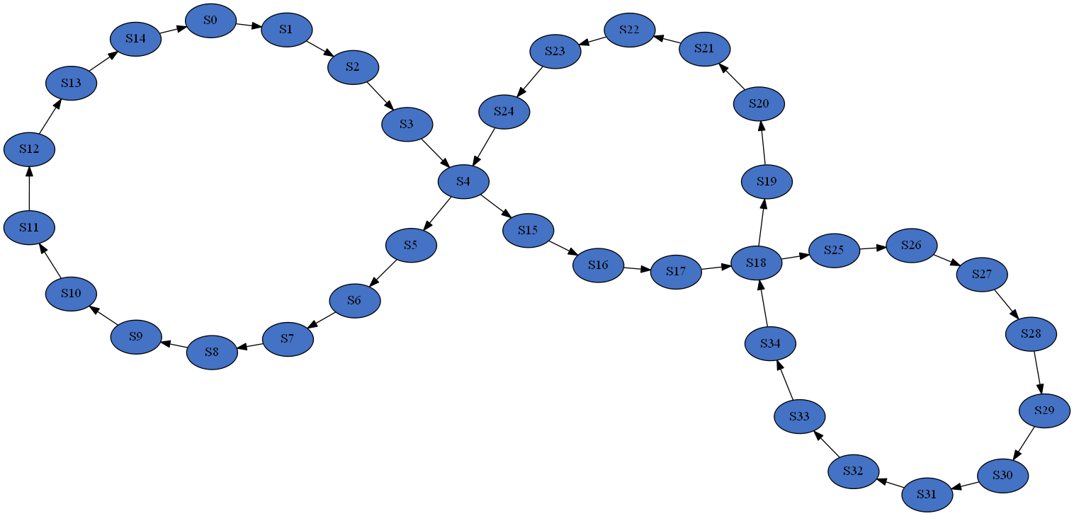
Cyclic
Cyclic networks can be constructed with
generate.cyclic(
    n_cycles=3,
    min_species=10,
    max_species=20,)
Three special arguments are available for cyclic models. n_cycles controls the number of cycles in the network.
min_species and max_species control the minimum and maximum number of nodes per cycle. The algorithm will
randomly sample from this range. The example below is a network with the above settings.
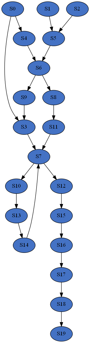
Branched
Branching networks can be constructed with
generate.branched(
    seeds=3,
    path_probs=[.1, .8, .1],
    tips=True,
)
Three special arguments are also available form branched networks. seeds is the number of starting nodes that
either split in two, grow linearly, or combine with another branch. path_probs is the probability of each of those
events happening at per iteration. And tips=True confines those events to the tips of the branches, i.e. the last
nodes in the growing branch(s) if grow or combine are chosen and the second to last node in one of the branches if
split is chosen. The example below is a network with the above settings.